This is a simple helical antenna calculator that I've been using for my antennas and dish feeds, originally I had it only in a private spreadsheet document. It is based on the book "Antennas For All Applications" by John D. Kraus and Ronald J. Marhefka and the "ARRL Antenna Book".
Scroll below the calculator to see more information about how to properly build a helix as well as explanations of its individual properties.
The beam width, gain, and impedance estimations are for informative purposes only, and may vary greatly from the real world performance of the antenna. It is even pointed out by John D. Kraus that the formulas tend to overestimate the gain. The estimates will become significantly less accurate as more turns are added to the antenna, or when very low or high turn spacing is used. They may also completely deviate from reality when using a different circumference. When some properties of the helix are exaggerated, the estimated gain may be very high and the beam very narrow while in the real world it is the exact opposite. Also, even at microwave frequencies, when the antenna is used near ground level its beam shape will depend a lot on its orientation and elevation. In practice this means that an antenna's beam may appear to be "deflected" away from its target.
The ground plane size is also not taken into account by this calculator, which is something that can greatly influence all of the mentioned values in the real world.
TL;DR: Keep your expectations realistic, if the theoretical performance shown by this calculator seems too good to be true, then it probably is. After building your helix, do a few tests to observe its performance and adjust it if necessary. For general purpose receive-only (or very low power transmit) applications based on already tested specifications, the estimations will be good enough.
Self-explanatory; F defines the frequency in MHz that the helix should operate at. At lower frequencies (below ~500 MHz), antennas such as the cross-dipole/cross-yagi are usually preferred for circular polarization due to the large scale of the helical antenna at those wavelengths. At high microwave frequencies (above ~3000 MHz), linear waveguide antennas and dish feeds with depolarizers become more convenient for DIY projects. Of course, when proper thought and care is given to the construction, helical antennas can work even outside of this range just fine, and in fact have been used in practice by amateurs and professionals alike (for example large helicals for the 2m ham band, or tiny ones for 5 GHz WiFi or drone/FPV use).
This is the vertical spacing between the turns of the helix expressed in wavelengths and millimeters respecitvely. For example, assuming a wavelength of 100 mm and Sλ of 0.1, the real turn spacing S would end up being 10 mm. Usually a turn spacing of 0.2 - 0.25 is recommended, though spacings as low as 0.1 are used in practice (for example most of my dish feeds use 0.14, while I have seen commercial Inmarsat antennas use around 0.1). When a lower spacing is used, the number of turns has to be increased accordingly to obtain the same gain and beamwidth.
The amount of turns (together with the turn spacing) is what defines the gain and beamwidth of the helical antenna - increasing the turn count also results in higher gain and directivity. In order for a helical antenna to work as intended, it needs to have at least ~3 turns. The highest turn count for a practical helix is ~16.
This is the circumference of an imaginary cylinder that the helix conductor is wound around (between conductor centers), expressed in wavelengths. The ideal value for a helical antenna is 1.0, though very small deviations may be used for experimenting.
Same as operating frequency F, except converted to wavelenght. Intermediary value used in other equations mainly for simplicity. For the purposes of this calculator, the wavelength is expressed in millimeters.
This is the value of Sλ expressed in millimeters according to the operational wavelength.
The diameter of the helical antenna, measured between the center points of the conductor.
Same as Sλ, except calculated for the current wavelength. This value together with diameter D are the two important measurements for constructing your helical antenna.
The half power beam width represents the angle within the main lobe of the antenna where its gain is above 50% of the peak gain (angle between -3dB points of the main lobe).
Similar to the half power beam width, except the first null angle is estimated between the points of the lowest gain around the main lobe (nulls).
Estimation of the peak gain of the helical antenna in dBi.
Estimation of the helical antenna's impedance. Normally this is around 140 Ω, though using a different circumference value will affect it. Information about easy impedance matching techniques can be found further down on this page.
Predicted total height of the helix. This does not include things like the ground plane or the connector that increase the total height, or impedance matching which can decrease the height.
This shows the angle at which the helical conductor is wound. When using a circumference Cλ of 1, it essentially expresses the same thing as the turn spacing Sλ. Similarly to the height A, this does not consider the pitch angle change in any impedance matching sections of the helix.
Length of conductor used for 1 normal turn of the helix.
This is an estimation of how much conductor (wire, tubing, ...) you will need to wind the helix. Once again, this does not consider things like impedance matching or build imperfections, so always leave yourself some extra length if you are cutting it beforehand.
This tells you which diameter to aim for when selecting your conductor to make the helix. As has been proven by many people though, it is not a critical design restriction, especially when using conductor thinner than recommended.
Estimated minimum diameter of a flat circular ground plane to achieve axial mode operation. In practice, square ground planes are often used, in which case the value can be treated as the minimum length of the square's side. Other ground plane types (such as "cups" or "cones") can be used to optimize the antenna's gain, beamwidth, and useful bandwidth.
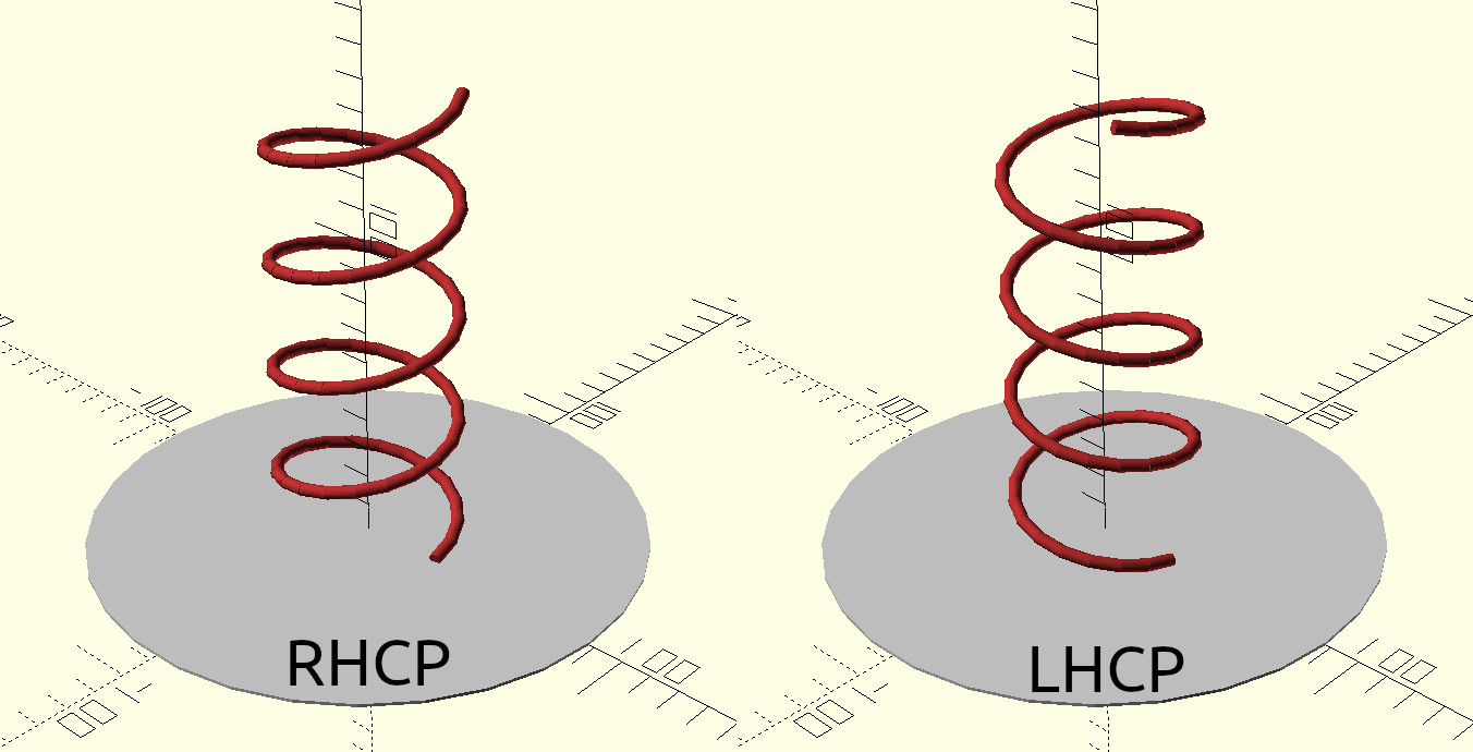
Depending on the way the helical conductor is wound, the resulting antenna will be either right-hand circularly polarized (RHCP) or left-hand circularly polarized (LHCP). A RHCP antenna will not be able to receive LHCP signals, while a LHCP antenna fails to receive RHCP. This is because of a theoretical infinite dB mismatch loss between RHCP and LHCP, although in the real world - where no antenna is perfect - even a RHCP helix will come with a (highly suppressed) LHCP component.
The polarization of a helix can be determined by looking down one of its ends; if the conductor turns in a clockwise manner then the helix is RHCP, if it is counter-clockwise then it's LHCP. As this can at first be confusing to imagine, I have created an image illustrating the visual difference between the two polarizations;
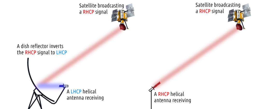
Continuing on the topic of polarization, one property of circularly polarized radio waves is that the polarization inverts when reflecting off a surface. This also includes the reflector of a dish antenna.
When using a helical antenna as a dish feed, it is important to use a helix polarization that is the opposite of the signal you want to receive. For example, if you want to receive a RHCP signal with your dish feeding a helix, then the helix has to be LHCP.
In the rare case of a dish reflector with additional subreflectors (Gregorian, Cassegrainian), the correct polarization flip has to be considered for each subreflector.
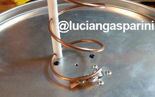
A helical antenna in a normal configuration has a high impedance of 140 ohms. Ideally this should be reduced close to 50 ohm to minimize the mismatch loss between the helix and the coaxial connector and cable. One simple way this can be done is by deforming a portion of the first turn so that its pitch gradually changes, from almost parallel to the ground plane to the nominal pitch of the rest of the helix.
Another common technique for helix impedance matching is adding a conductive strip to the first quarter turn, this increases the helix conductor's surface area and forms a "capacitor" with the ground plane.
An example of a helical antenna utilizing both methods can be seen below.